Problem set 1
Due by 11:59 PM on Tuesday, September 18, 2018
Task 0
Download this R Markdown file.Your browser might show the file instead of downloading it. If that’s the case, you can copy/paste the code from the browser to RStudio. In RStudio, go to “File” > “New” > “New R Markdown…”, click “OK” with the default options, delete all the placeholder code/text in the new file, and paste the example code in the now-blank file.
It contains an outline/skeleton of what you’ll need to do in this problem set, and it includes lots of the code prewritten just for you!
Make sure you install R and RStudio and tidyverse first.Follow these instructions and install R, RStudio, and all the tidyverse packages. If you have any questions, don’t hesitate to ask me or your classmates for help!
Complete the three tasks below and type your answers in that downloaded file. When you’re done, knit the document as a Word file or PDF with the “Knit” button at the top of the script editing pane.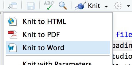
Task 1: Become familiar with RStudio and R Markdown
In Task 2, you’ll play with actual R commands and create graphics. Before we get there, you need to familiarize yourself with RStudio. Go through this short tutorial.
Finally, you will write future memos and problems sets in R Markdown instead of Word. RStudio has a helpful tutorial and a short video about R Markdown. Go through these short lessons:
- Introduction
- How it Works
- Code Chunks
- Inline Code
- Markdown Basics The R Markdown Reference Guide is super useful here.
- Output Formats
Before doing these R Markdown tutorials, you’ll need to install a couple more R packages. Use RStudio’s “Packages” panel to install rmarkdown and viridis. Alternatively, paste these commands in the RStudio Console: install.packages("rmarkdown") and install.packages("viridis"). You can also type install.packages(c("rmarkdown", "viridis")) to install both at the same time.
Don’t worry if you don’t completely understand R Markdown! We’ll go over it at the beginning of class next Tuesday. Try your hardest and play around with it.
Also, if you want to convert R Markdown files to PDF instead of just Word or HTML (which you do), you’ll need to install LaTeX, which is a fancy scientific typesetting program. You don’t need to know how it works—it just has to be installed for R to use it.
The easiest way to install it is with the tinytex R package. Run these two lines in your R console to install a smaller version of LaTeX that should work great for this class:
install.packages('tinytex')
tinytex::install_tinytex()
If you want to use a full-blown LaTeX installation, install one of these. But note that you don’t need to do this!
- LaTeX for macOS: MacTeX For whatever reason, LaTeX is astoundingly huge and it will feel like you’re downloading the entire internet when you install it. Be patient :)
- LaTeX for Windows: MiKTeX
When you’re done with everything in Task 1, type something in the R Markdown skeleton file you downloaded at the beginning. You should see a # Task 1 heading. Type it under that.
Task 2: Playing with R
This example uses data from the Gapminder project.
You may have seen Hans Rosling’s delightful TED talk showing how global health and wealth have been increasing. If you haven’t, you should watch it. Sadly, Hans died in February 2017.
You’ll need to install the gapminder R package first. Install it either with the “Packages” panel in RStudio or by typing install.packages("gapminder") in the R console.
For this task, you won’t do any actual coding. The skeleton R Markdown file has all the code you need for this task. Download it, open it in RStudio, and walk through the examples in RStudio on your computer. If you place your cursor on some R code and press “⌘ + enter” (for macOS users) or “ctrl + enter” (for Windows users), RStudio will send that line to the console and run it.
There are a few questions that you’ll need to answer, but that’s all. Those are marked with “TYPE YOUR ANSWER HERE.”
Task 3: R and ggplot2
Read Chapter 3 of R for Data Science and complete the following exercises:
- 3.2.4: Questions 1–5
- 3.3.1: Questions 1–5
- 3.5.1: Questions 1–4
- 3.6.1: Questions 1–5 (#6 if you’re feeling adventurous)
- 3.8.1: Questions 1 and 2
All done!
Knit the completed R Markdown file as a Word document or PDF (use the “Knit” button at the top of the script editor window) and upload it to Learning Suite.