Space

Materials for class on Tuesday, November 6, 2018

Slides
Installing sf and other GIS software
Projections and coordinate reference systems
Shapefiles to download
Live code
Examples of using the sf library
Clearest and muddiest things

Slides

Download the slides from today’s lecture.

Installing `sf` and other GIS software

Plotting geographic stuff with ggplot is easy nowadays with the new sf package, which works nicely within the tidyverse paradigm. Using the “Packages” panel in RStudio, install these packages: sf, maps, maptools, and rgeos
Extra step for macOS people only: R doesn’t do all the geographic calculations by itself—it relies on a few pieces of standalone GIS software behind the scenes. When people on Windows install sf, those pieces of software should be installed automatically. This doesn’t happen on macOS, so you have to install them manually. The easiest way to do this is with Terminal. Here’s what you have to do:
1. Open Terminal
2. Type xcode-select --install
  
  A software update popup window should appear that will ask if you want to install command line developer tools. Click on “Install” (you don’t need to click on “Get Xcode”)
3. Go to brew.sh, copy the big long command under “Install Homebrew” (starts with /usr/bin/ruby -e "$(curl -fsSL...), paste it into Terminal, and press enter. This installs Homebrew, which is special software that lets you install Unix-y programs from the terminal.⊕ You can install stuff like MySQL, Python, Apache, and even R if you want; there’s a full list of Homebrew formulae here.
4. Type this line in Terminal to install gdal, geos, and proj:
```
 brew install gdal geos proj udunits
```
5. Wait for a few minutes while all that stuff compiles.
Verify that this all worked by running library(sf) in RStudio. You should see a message saying something like Linking to GEOS 3.6.1, GDAL 2.1.3, proj.4 4.9.3. That means it’s working.

Projections and coordinate reference systems

As you read in this week’s readings, projections matter a lot for maps. You can convert your geographic data between different coordinate systems (or projections)TECHNICALLY coordinate systems and projection systems are different things, but I’m not a geographer and I don’t care that much about the nuance.

fairly easily with sf. You can use coord_sf(crs = st_crs(XXXX)) to convert coordinate reference systems (CRS) as you plot, or use st_transform() to convert data frames to a different CRS.

There are standard indexes of more than 4,000 of these projections (!!!) at spatialreference.org or at epsg.io. Here are some common ones:

54002: Equidistant cylindrical projection for the worldThis is essentially the Gall-Peters projection from the West Wing clip.
54004: Mercator projection for the world
54008: Sinusoidal projection for the world
54009: Mollweide projection for the world
54030: Robinson projection for the worldThis is my favorite world projection.
4326: WGS 84: DOD GPS coordinates (standard -180 to 180 system)
4269: NAD 83: Relatively common projection for North America
102003: Albers projection specifically for the contiguous United States

Alternatively, instead of using these index numbers, you can use any of the names listed at proj.4, such as:

st_crs("+proj=merc"): Mercator
"+proj=robin": Robinson
"+proj=moll": Mollweide
"+proj=aeqd": Azimuthal Equidistant
"+proj=cass": Cassini-Soldner

Shapefiles to download

Download and unzip these and put them in a folder named “data” in a new RStudio project:

Live code

Use this link to see the code that I’m actually typing:

https://andhs.co/live-code

I’ve saved the R script to Dropbox, and that link goes to a live version of that file. Refresh or re-open the link as needed to copy/paste code I type up on the screen.

Examples of using the `sf` library

First we load the packages we’ll be using:

library(tidyverse)
library(sf)
library(scico)

Load shapefiles

And then we load a bunch of shapefiles. You downloaded these from the links up above. This assumes they’re in a folder named data, with each collection of shapefile stuff in its own subfolder. The stringsAsFactors option makes it so any character-based columns are loaded as actual text data instead of as a factor. You can also use read_sf() to read these shapefiles without neeing to set stringsAsFactors = FALSE

# Load all these shapefiles!
# https://gis.utah.gov/data/boundaries/citycountystate/
utah_counties <- st_read("data/Counties/Counties.shp",
                         stringsAsFactors = FALSE)

# https://gis.utah.gov/data/society/schools-libraries/
utah_libraries <- st_read("data/Libraries/Libraries.shp",
                          stringsAsFactors = FALSE)

# https://gis.utah.gov/data/society/places-of-worship/
utah_places_of_worship <- st_read("data/PlacesOfWorship/PlacesOfWorship.shp",
                                  stringsAsFactors = FALSE)

# https://www.census.gov/geo/maps-data/data/cbf/cbf_state.html
us_states <- st_read("data/cb_2017_us_state_20m/cb_2017_us_state_20m.shp",
                     stringsAsFactors = FALSE)

# https://www.naturalearthdata.com/downloads/110m-cultural-vectors/
countries <- st_read("data/ne_110m_admin_0_countries/ne_110m_admin_0_countries.shp",
                     stringsAsFactors = FALSE)

Wrangle and clean data

Because st_read() (or read_sf()) loads these shapefiles as data frames, all our typical dplyr verbs work (like mutate(), filter(), group_by(), etc.). Let’s clean up a couple of these datasets:

# Only look at contiguous US
states_48 <- us_states %>% 
  filter(!(STUSPS %in% c("HI", "AK", "PR")))

# Omit Antarctica
countries_with_people <- countries %>% 
  filter(ISO_A3 != "ATA")

World map with different projections

Making a map is really as simple as using geom_sf(). This is so magical.

ggplot() +
  geom_sf(data = countries_with_people)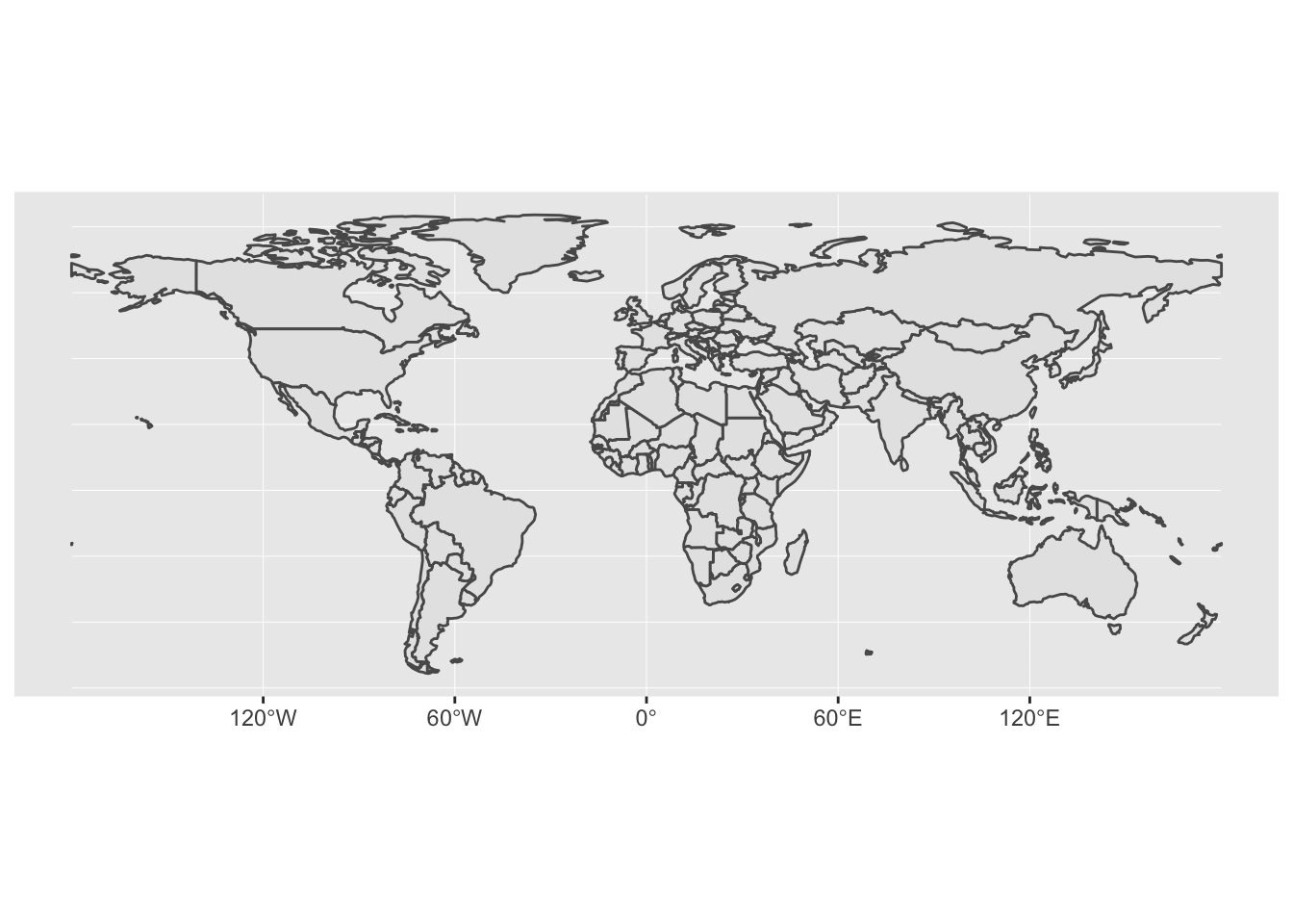

We can change the projection of the map with coord_sf() and specify different coordinate reference systems (CRS). See above for a list of a bunch of different ones. Also, because geom_sf() is a standard ggplot layer, we assign it fills and colors and sizes and alphas and anything else you can do with a geom_*() layer.

Also, the Natural Earth data conveniently includes columns indicating a country’s continent (CONTINENT), as well as a coloring scheme with 7–13 colors (MAPCOLOR7, MAPCOLOR9, etc.) so that no countries with a shared border share a color.

Here are a bunch of maps colored differently and with different projections:

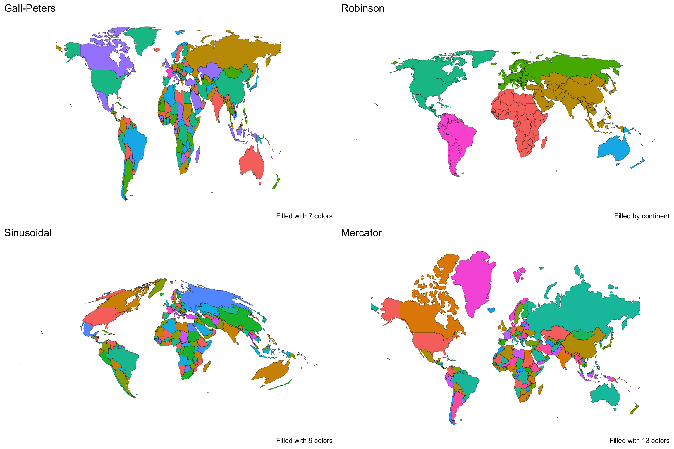
US map with different projections

The map of the US can also be projected differently—two common projections are NAD83 and Albers.

Unfortunately the shapefile from the Census doesn’t include a cool column for state colors. BUUUUT I found a map somebody made on Flickr with 4 colors, and they included a list of color divisions, so I copied that list and made a mini data frame of it.

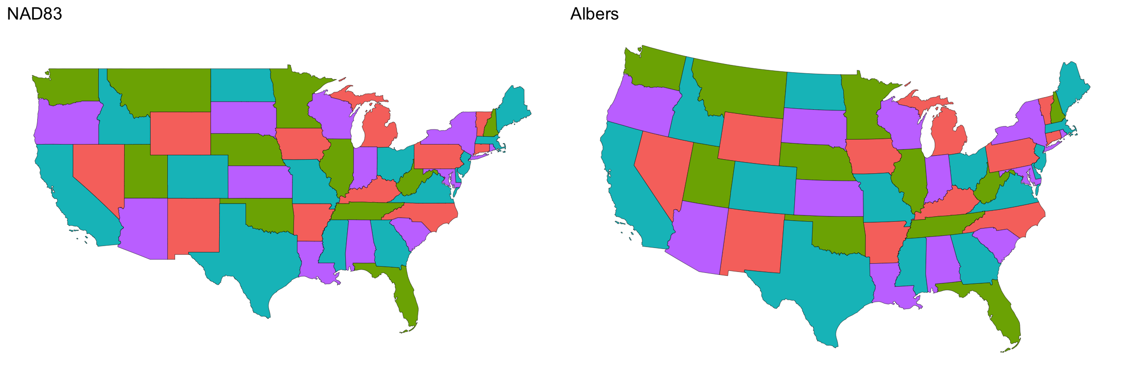
Plotting libraries and counties

The geom_sf() function is smart enough to adapt to the type of data in the magic geometry column in the shapefile. If the geometry is a polygon, like country or state shapes, it’ll make a polygon. If the geometry is a bunch of x, y coordinates, it’ll make points. Here’s an example of using geom_sf() to make both county shapes and points marking libraries.

Also, again because these shapefiles are essentially data frames, we can use standard dplyr verbs on them, like group_by() and summarize().

# Calculate the count of libraries per county
libraries_per_county <- utah_libraries %>%
  group_by(COUNTY) %>%
  summarize(num_libraries = n()) %>%
  # Change the NAME column to upper case so that it can join with the utah_counties data frame
  mutate(NAME = str_to_upper(COUNTY))

utah_counties_with_libraries <- utah_counties %>%
  # Join the summarized libraries-per-county data
  st_join(libraries_per_county) %>%
  # Calculate the number of libraries per capita
  mutate(people_per_library = POP_CURRES / num_libraries)

# Plot both of these with geom_sf
ggplot() +
  # This will plot the counties
  geom_sf(data = utah_counties_with_libraries, 
          aes(fill = people_per_library), size = 0.25) +
  # This will plot the libraries as points
  geom_sf(data = libraries_per_county, size = 0.5) +
  coord_sf(crs = 26912, datum = NA) +  # 26912 is NAD83, but specifically for North America
  scale_fill_scico(palette = "bilbao", end = 0.9, begin = 0.05,
                   labels = scales::comma, na.value = "white",
                   name = "People per library") +
  guides(fill = guide_colorbar(barwidth = 10, barheight = 1)) +
  labs(title = "Libraries in Utah",
       subtitle = "Davis and Weber counties seem to be the most\nunderserved given their populations") +
  theme_void() +
  theme(legend.position = "bottom",
        plot.title = element_text(face = "bold"))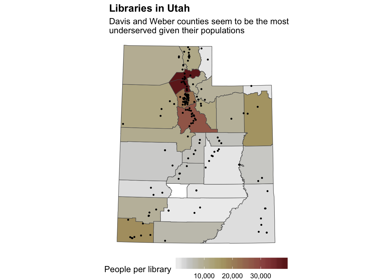

Converting to different projections

So far we’ve converted to different projections as we plot using coord_sf(). This forces all the geom_sf() layers to use the same CRS, regardless of what their geometry columns are currently using.

Alternatively, you can make the CRS conversion within the data frame itself with st_transform(). This is useful for situations where you might want to plot things without geom_sf(), like adding labels with geom_label(), since your x and y coordinates need to be in the same projection as your other map elements.

libraries_albers <- utah_libraries %>% 
  st_transform(102003)

libraries_albers %>% pull(geometry) %>% head()

## Geometry set for 6 features 
## geometry type:  POINT
## dimension:      XY
## bbox:           xmin: -1434813 ymin: 212729 xmax: -1250077 ymax: 579980.8
## epsg (SRID):    102003
## proj4string:    +proj=aea +lat_1=29.5 +lat_2=45.5 +lat_0=37.5 +lon_0=-96 +x_0=0 +y_0=0 +datum=NAD83 +units=m +no_defs
## First 5 geometries:

## POINT (-1323639 432520.5)

## POINT (-1434813 212729)

## POINT (-1324264 549928.3)

## POINT (-1320397 560885.8)

## POINT (-1300693 579980.8)

libraries_gps <- utah_libraries %>% 
  st_transform(4326)

libraries_gps %>% pull(geometry) %>% head()

## Geometry set for 6 features 
## geometry type:  POINT
## dimension:      XY
## bbox:           xmin: -112.6421 ymin: 38.27423 xmax: -110.7378 ymax: 41.70823
## epsg (SRID):    4326
## proj4string:    +proj=longlat +datum=WGS84 +no_defs
## First 5 geometries:

## POINT (-111.7966 40.37548)

## POINT (-112.6421 38.27423)

## POINT (-112.0381 41.40833)

## POINT (-112.0143 41.51064)

## POINT (-111.818 41.70823)

Making your own geoencoded data

You don’t have to rely on shapefiles you find on the internet for all your geographic plotting needs. You can make your own data! Here, I found the latitude and longitude for three cities in Utah with Google Maps.Right click anywhere in Google Maps, select “What’s here?”, and see the exact coordinates for that spot.

I made this data frame with tribble(), but you could also put these in a CSV file (or even have them in a CSV file already, like with the rat data from mini project 1).

The st_as_sf() function converts the two columns into a magic geometry column based on the projection you feed it. In this case, 4326 is the standard -180 to 180 lat/lon system used by GPSes and Google Maps.

city_data <- tribble(
  ~city, ~long, ~lat,
  "Provo", -111.652327, 40.250396,
  "Salt Lake City", -111.921267, 40.755425,
  "Moab", -109.553448, 38.572405
) %>% 
  st_as_sf(coords = c("long", "lat"), crs = 4326) 

city_data

## Simple feature collection with 3 features and 1 field
## geometry type:  POINT
## dimension:      XY
## bbox:           xmin: -111.9213 ymin: 38.57241 xmax: -109.5534 ymax: 40.75543
## epsg (SRID):    4326
## proj4string:    +proj=longlat +datum=WGS84 +no_defs
## # A tibble: 3 x 2
##   city                       geometry
##   <chr>                   <POINT [°]>
## 1 Provo           (-111.6523 40.2504)
## 2 Salt Lake City (-111.9213 40.75543)
## 3 Moab           (-109.5534 38.57241)

This city_data object is now essentially a shapefile that is plottable with geom_sf(). Also, notice how even though utah_shape and city_data use different CRSes, coord_sf() forces them to plot using the same NAD83 26912 CRS.

# Extract Utah out of the states_48 data
utah_shape <- states_48 %>% 
  filter(STUSPS == "UT")

ggplot() +
  geom_sf(data = utah_shape, fill = "lightblue") +
  geom_sf(data = city_data) +
  coord_sf(crs = 26912, datum = NA) +
  theme_void()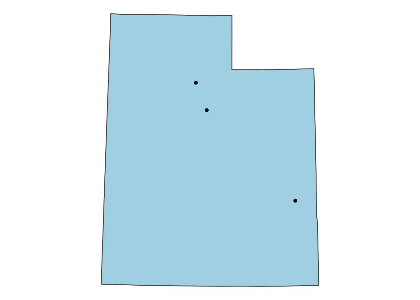

We can add labels here too, but first we need a little bit of trickery. geom_sf() doesn’t handle labels, so we need to use our normal geom_label() function, which means we need an x and y value. As it stands now, we have an x and a y (longitude and latitude), but those values are stuck in the magic geometry column. We can extract them using the st_coordinates() function:

city_data_with_xy <- city_data %>% 
  mutate(long = st_coordinates(.)[,1],
         lat = st_coordinates(.)[,2])
city_data_with_xy

## Simple feature collection with 3 features and 3 fields
## geometry type:  POINT
## dimension:      XY
## bbox:           xmin: -111.9213 ymin: 38.57241 xmax: -109.5534 ymax: 40.75543
## epsg (SRID):    4326
## proj4string:    +proj=longlat +datum=WGS84 +no_defs
## # A tibble: 3 x 4
##   city            long   lat             geometry
##   <chr>          <dbl> <dbl>          <POINT [°]>
## 1 Provo          -112.  40.3  (-111.6523 40.2504)
## 2 Salt Lake City -112.  40.8 (-111.9213 40.75543)
## 3 Moab           -110.  38.6 (-109.5534 38.57241)

Neat! The one problem, though, is that it extracts them using whatever CRS the geometry column is currently set to. Here it’s 4326 (the Google Maps form), but if we want to use NAD83 (26912), these x and y points won’t work. We need to convert the geometry column to our desired final CRS before extracting the points. Notice how these points now are in the hundreds of thousands instead of between -180 and 180:

city_data_with_xy <- city_data %>% 
  st_transform(26912) %>% 
  mutate(long = st_coordinates(.)[,1],
         lat = st_coordinates(.)[,2])
city_data_with_xy

## Simple feature collection with 3 features and 3 fields
## geometry type:  POINT
## dimension:      XY
## bbox:           xmin: 422233.8 ymin: 4270320 xmax: 626012.9 ymax: 4512016
## epsg (SRID):    26912
## proj4string:    +proj=utm +zone=12 +ellps=GRS80 +towgs84=0,0,0,0,0,0,0 +units=m +no_defs
## # A tibble: 3 x 4
##   city              long      lat           geometry
##   <chr>            <dbl>    <dbl>        <POINT [m]>
## 1 Provo          444521. 4455753. (444521.3 4455753)
## 2 Salt Lake City 422234. 4512016. (422233.8 4512016)
## 3 Moab           626013. 4270320. (626012.9 4270320)

With this numeric longitude and latitude, we can plot this data with regular geom_*() functions:

ggplot() +
  geom_sf(data = utah_shape, fill = "lightblue") +
  geom_sf(data = city_data_with_xy) +
  # This nudge value has to be huge because NAD83 uses giant numbers. If we were
  # plotting with the Google Maps 4326, we'd only need to nudge a little bit
  geom_label(data = city_data_with_xy, aes(x = long, y = lat, label = city),
             nudge_y = 25000) +  
  # This forces the two geom_sf layers to use 26912, but doesn't affect
  # geom_label; we took care of that by hand
  coord_sf(crs = 26912, datum = NA) +
  theme_void()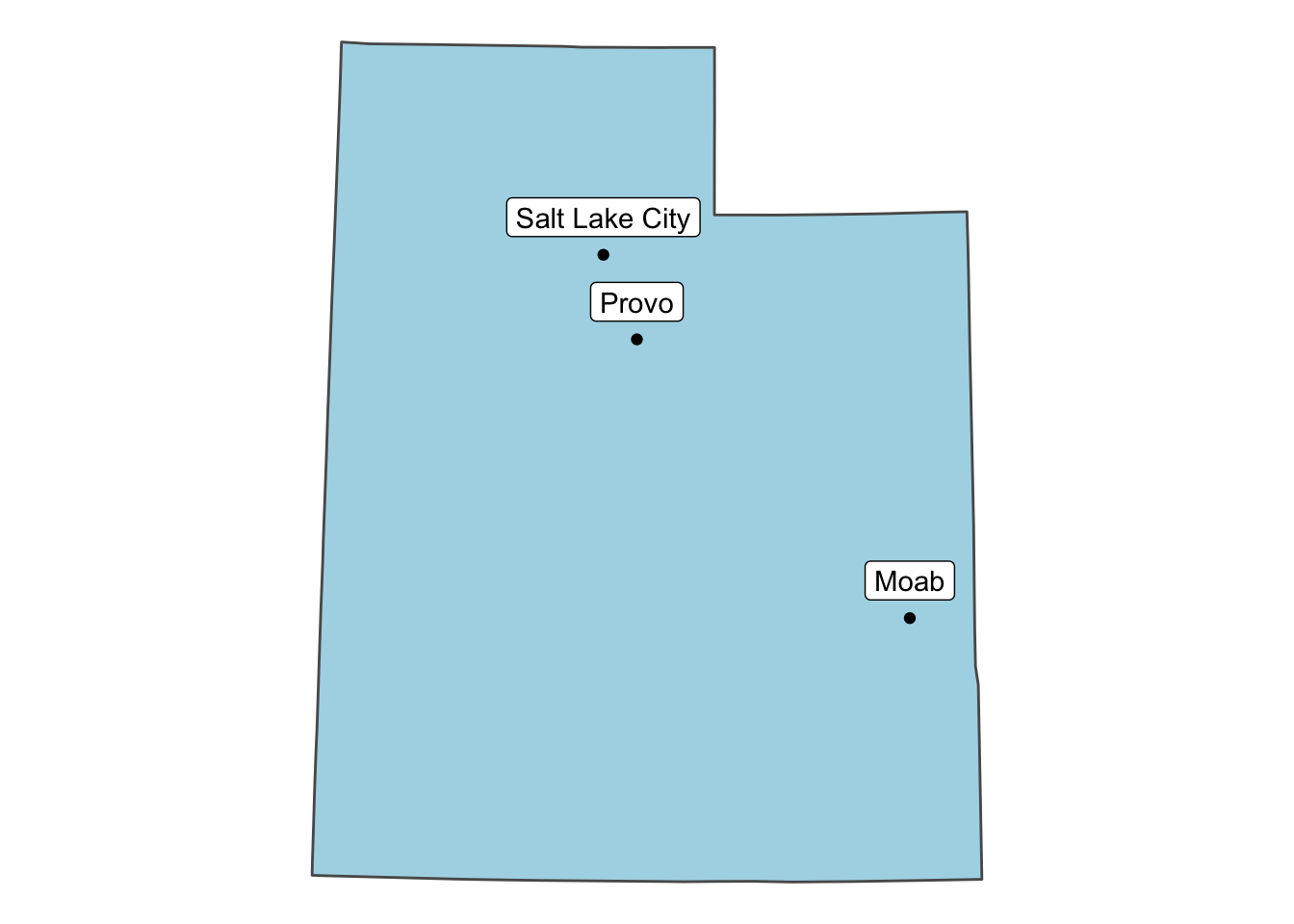

Centroids

We didn’t cover this in class, but it’s helpful to know. You can use the st_centroid() function to find the middle of a polygon. This is helpful if you want to add labels to counties or states and put them in the middle without looking up their coordinates in Google Maps. Because you use geom_label() or geom_text() to plot the labels, you need to extract the coordinates like we did above, but that’s fairly trivial. Here’s the Utah libraries map with labels in the center of each county.

# Find county centroids
counties_centroid <- utah_counties %>% 
  # Convert geometry column to NAD83, since that's what we use in the final plot
  st_transform(26912) %>% 
  # Calculate centroid points for every county
  st_centroid() %>% 
  # Extract these as actual numbers
  mutate(long = st_coordinates(.)[,1],
         lat = st_coordinates(.)[,2]) %>% 
  # Make the county names title case instead of ALL CAPS
  mutate(NAME = str_to_title(NAME))
# This will probably give you a warning. I don't know why, but it still works in
# the end, so you can ignore it I guess


ggplot() +
  # This will plot the counties
  geom_sf(data = utah_counties_with_libraries, 
          aes(fill = people_per_library), size = 0.25) +
  # This will plot the libraries as points
  geom_sf(data = libraries_per_county, size = 0.5) +
  # This will add the county labels
  geom_label(data = counties_centroid, aes(x = long, y = lat, label = NAME),
             size = 2, alpha = 0.25) +
  coord_sf(crs = 26912, datum = NA) +  # 26912 is NAD83, but specifically for North America
  scale_fill_scico(palette = "bilbao", end = 0.9, begin = 0.05,
                   labels = scales::comma, na.value = "white",
                   name = "People per library") +
  guides(fill = guide_colorbar(barwidth = 10, barheight = 1)) +
  labs(title = "Libraries in Utah",
       subtitle = "Davis and Weber counties seem to be the most\nunderserved given their populations") +
  theme_void() +
  theme(legend.position = "bottom",
        plot.title = element_text(face = "bold"))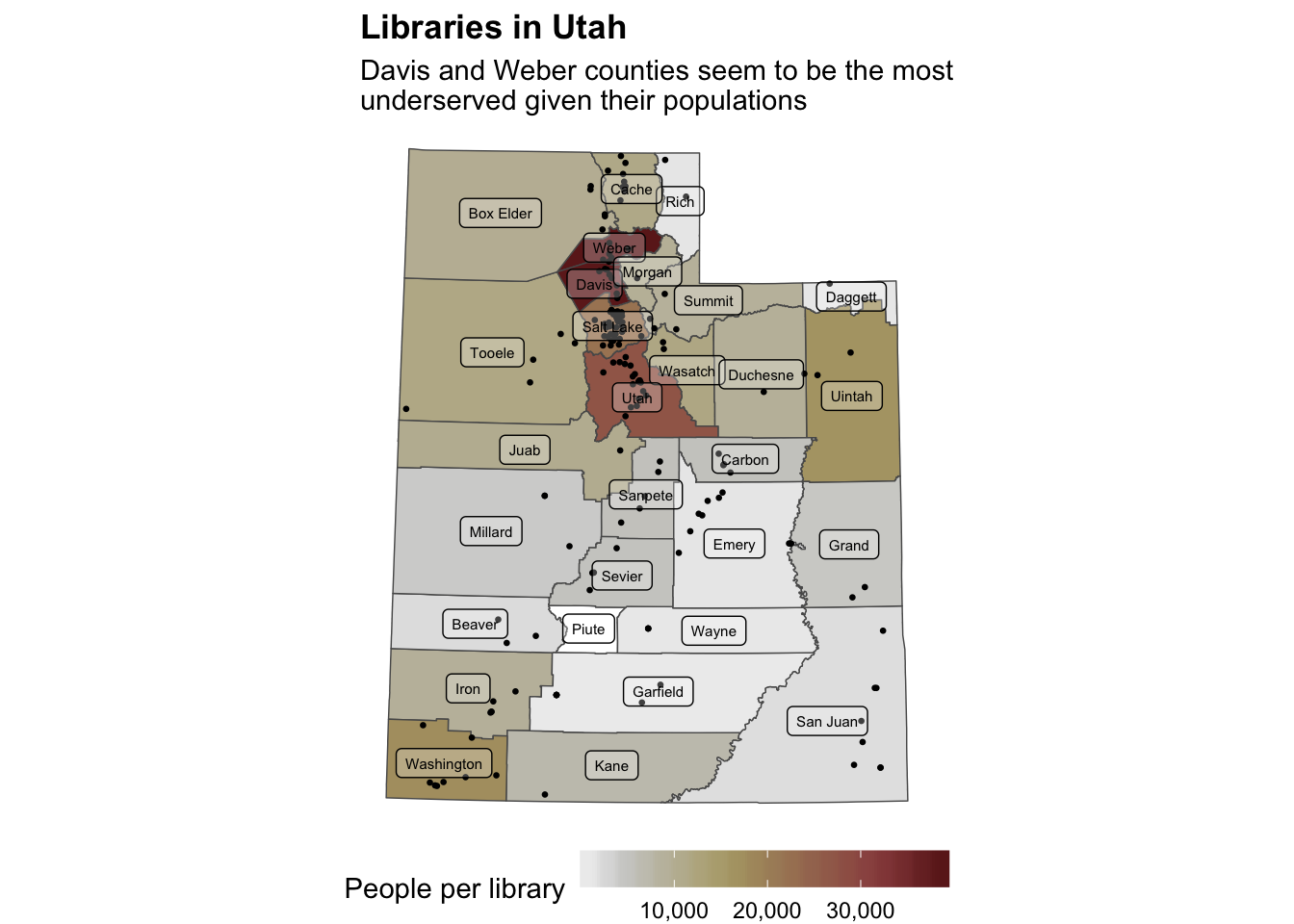

So cool!

Clearest and muddiest things

Go to this form and answer these two questions:

What was the muddiest thing from class today? What are you still wondering about?
What was the clearest thing from class today? What was the most exciting thing you learned?

I’ll compile the questions and send out answers after class.