Text

Materials for class on Tuesday, November 13, 2018

Slides
Data to download
Live code
Tidy text analysis
Clearest and muddiest things

Slides

Download the slides from today’s lecture.

Data to download

Download these and put them in a folder named “data” in an RStudio project:

Live code

Use this link to see the code that I’m actually typing:

https://andhs.co/live-code

I’ve saved the R script to Dropbox, and that link goes to a live version of that file. Refresh or re-open the link as needed to copy/paste code I type up on the screen.

Tidy text analysis

In class, we looked at a bunch of different methods for analyzing text. At the foundation of all this text analysis, all we’re really doing is counting words in fancy ways. This stuff isn’t magic—it’s just counting.

We’ll start by loading the libraries we’ll need, as well as the data linked above.

library(tidyverse)
library(tidytext)
library(gutenbergr)
library(topicmodels)
library(textfeatures)

# For cool natural language processing; go to
# https://statsmaths.github.io/cleanNLP/ for documentation and examples
library(cleanNLP)

# Text from http://scriptures.nephi.org/
scriptures <- read_csv("data/lds-scriptures.csv") %>% 
  select(volume_title, book_title, chapter_number, verse_number, scripture_text)

# Get just the Book of Mormon and make sure the book names are in order
bom <- scriptures %>% 
  filter(volume_title == "Book of Mormon") %>% 
  mutate(book_title = fct_inorder(book_title))

# Get just the OT and NT
bible <- scriptures %>% 
  filter(volume_title %in% c("Old Testament", "New Testament"))

# Download 4 Dickens books
dickens <- gutenberg_download(c(19337, 98, 1400, 766),
                              meta_fields = "title")

# Load the pre-parts-of-speechified BoM so you don't have to run the tagger yourself
bom_annotated <- read_csv("data/bom_annotated.csv")

Part-of-speech tagging

When you first work with text in R, R has no way of knowing if words are nouns, verbs, or adjectives. You can algorithmically predict what part of speech each word is using a part-of-speech tagger, like spaCy or Stanford NLP. You can do this in R with the cleanNLP package, which connects to external natural language processing algorithms like spaCy or Stanford’s thing.

Installing cleanNLP is trivial—it’s just a normal R package, so use the “Packages” panel in RStudio—but connecting it with external NLP algorithms is a little trickier. To install spaCy, which is a really fast tagging library, do this:

Make sure Python is installed (it is if you’re on macOS or Linux; good luck with Windows—I have no idea how to install this stuff there, but there’s a way).
Open Terminal and run this command to install spaCy:
```
pip install -U spacy
```
Run this command to download spaCy’s English algorithms:
```
python -m spacy download en
```
The end!

Here’s the general process for tagging (they call it annotating) text:

Make a dataset where the first column is the id (line number, chapter number, book+chapter, whatever) and the second column is the text itself.
Initialize the NLP tagger. You can use an R-only one that doesn’t need Python or any other external dependencies with cnlp_init_udpipe(). If you’ve installed spaCy, use cnlp_init_spacy(). If you’ve installed Stanford’s thing, use cnlp_init_corenlp().
Feed the data frame from step 1 into the cnlp_annotate() function and wait.
Save the tagged data as a file on your computer so you don’t have to retag it every time. Use cnlp_get_tif() %>% write_csv().
The end!

# Wrangle BoM text into format that cnlp_annotate() needs
bom_chapters <- bom %>%
  mutate(book_chapter = paste(book_title, chapter_number)) %>%
  select(book_title, book_chapter, scripture_text) %>%
  nest(scripture_text) %>%
  mutate(text = data %>% map_chr(~ paste(.$scripture_text, collapse = " "))) %>%
  select(book_chapter, text, book_title)

# Set up NLP backend
# cnlp_init_udpipe()  # This NLP engine doesn't need Python, but it's so so so slow
cnlp_init_spacy()  # Use spaCy

# Tag all the parts of speech!
bom_annotated <- cnlp_annotate(bom_chapters, as_strings = TRUE)

# Save the tagged data so we don't have to tag it all again
cnlp_get_tif(bom_annotated) %>%
  write_csv(path = "data/bom_annotated.csv")

Tokens and word counts

Single words

Now that we have tidy text, we can start counting words. Here’s what’s happening below:

We use unnest_tokens() to split each verse (in this case each row is a verse; that’s not always the case, though—sometimes it’ll be chapters or lines or entire books) into separate words.
We use anti_join() to remove all the common stop words like “a” and “the”. You can do the same thing with filter() like so: filter(!(word %in% stop_words$word)) (I prefer this way, actually)
We count how many times each word appears and sort the list
We keep just the top 15 words
We plot it with geom_col()

bom_words <- bom %>% 
  unnest_tokens(word, scripture_text) %>% 
  anti_join(stop_words) %>% 
  # count(book_title, word, sort = TRUE)
  count(word, sort = TRUE) %>% 
  top_n(15) %>% 
  mutate(word = fct_inorder(word))

ggplot(bom_words, aes(x = fct_rev(word), y = n)) + 
  geom_col() + 
  coord_flip() +
  scale_y_continuous(labels = scales::comma) +
  labs(y = "Count", x = NULL, title = "15 most frequent words in the Book of Mormon") +
  theme_minimal()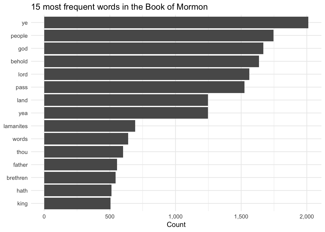

Bigrams

We can also look at the frequency of pairs of words. First we’ll look at common bigrams, filtering out stop words again (since we don’t want things like “of the” and “in the”):

bom_bigrams <- bom %>% 
  unnest_tokens(bigram, scripture_text, token = "ngrams", n = 2) %>% 
  # Split the bigram column into two columns
  separate(bigram, c("word1", "word2"), sep = " ") %>% 
  filter(!word1 %in% stop_words$word,
         !word2 %in% stop_words$word) %>% 
  # Put the two word columns back together
  unite(bigram, word1, word2, sep = " ") %>% 
  count(bigram, sort = TRUE) %>% 
  top_n(10)

# We could plot this bom_bigrams object with geom_col(), but I'll skip that part
# Here's what this looks like:
bom_bigrams

## # A tibble: 10 x 2
##    bigram               n
##    <chr>            <int>
##  1 thou hast          127
##  2 lord god           115
##  3 holy ghost          94
##  4 thou shalt          94
##  5 lord hath           67
##  6 jesus christ        66
##  7 beloved brethren    65
##  8 thou art            57
##  9 judgment seat       54
## 10 behold ye           49

Bigrams and probability

We can replicate the “She Giggles, He Gallops” idea by counting the bigrams that match “he X” and “she X”.

The log ratio idea shows how much more likely a word is compared to its counterpart (so “she fled” is more than 4x more likely to appear than “he fled”. In this graph, I replaced the x-axis labels with “2x” and “4x”, but without those, you get numbers like 1, 2, and 3 (or -1, -2, -3)). To convert those logged ratio numbers into the multiplicative version (i.e. 2x instead of 1), raise 2 to the power of the log ratio. If the log ratio is 3, the human-readable version is $2^3$, or 8 times.

# Take the log of 8:
log2(8)

## [1] 3

# Reverse log of 3:
2^3

## [1] 8

The only text wizardry here is tokenizing the words. Pretty much the rest of all this code is just dplyr mutating, filtering, and counting:

pronouns <- c("he", "she")

bigram_he_she_counts <- bom %>%
  unnest_tokens(bigram, scripture_text, token = "ngrams", n = 2) %>%
  count(bigram, sort = TRUE) %>%
  # Split the bigram column into two columns
  separate(bigram, c("word1", "word2"), sep = " ") %>%
  # Only choose rows where the first word is he or she
  filter(word1 %in% pronouns) %>%
  count(word1, word2, wt = n, sort = TRUE) %>%
  rename(total = nn)

word_ratios <- bigram_he_she_counts %>%
  # Look at each of the second words
  group_by(word2) %>%
  # Only choose rows where the second word appears more than 10 times
  filter(sum(total) > 10) %>%
  ungroup() %>%
  # Spread out the word1 column so that there's a column named "he" and one named "she"
  spread(word1, total, fill = 0) %>%
  # Add 1 to each number so that logs work (just in case any are zero)
  mutate_if(is.numeric, funs((. + 1) / sum(. + 1))) %>%
  # Create a new column that is the logged ratio of the she counts to he counts
  mutate(logratio = log2(she / he)) %>%
  # Sort by that ratio
  arrange(desc(logratio))

# Rearrange this data so it's plottable
plot_word_ratios <- word_ratios %>%
  # This gets the words in the right order---we take the absolute value, select
  # only rows where the log ratio is bigger than 0, and then take the top 15 words
  mutate(abslogratio = abs(logratio)) %>%
  group_by(logratio < 0) %>%
  top_n(15, abslogratio) %>%
  ungroup() %>%
  mutate(word = reorder(word2, logratio)) 

# Finally we plot this
ggplot(plot_word_ratios, aes(word, logratio, color = logratio < 0)) +
  geom_segment(aes(x = word, xend = word,
                   y = 0, yend = logratio), 
               size = 1.1, alpha = 0.6) +
  geom_point(size = 3.5) +
  coord_flip() +
  labs(y = "How much more/less likely", x = NULL) +
  scale_color_discrete(name = "", labels = c("More 'she'", "More 'he'")) +
  scale_y_continuous(breaks = seq(-3, 3),
                     labels = c("8x", "4x", "2x",
                                "Same", "2x", "4x", "8x")) +
  theme_minimal() +
  theme(legend.position = "bottom")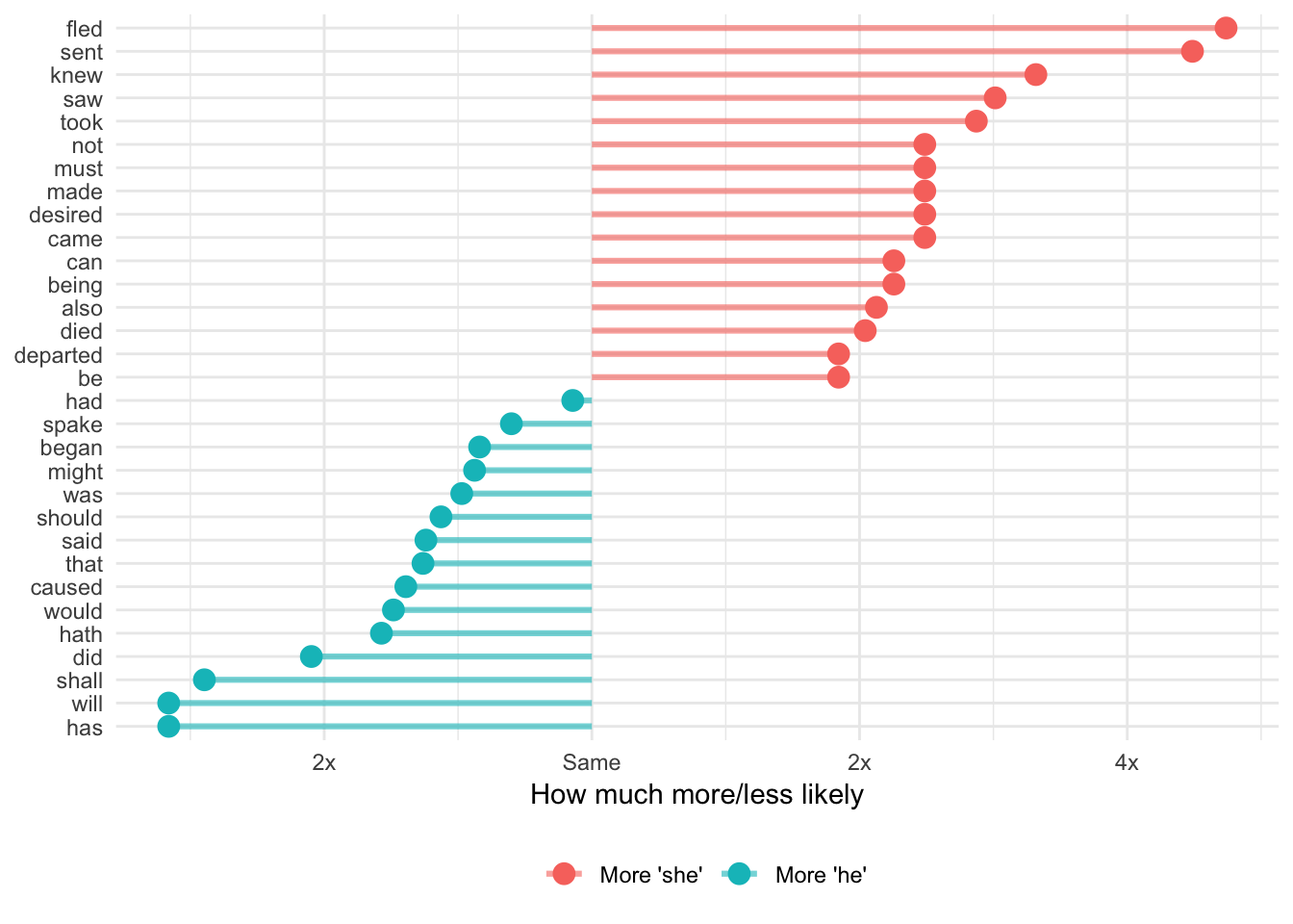

Sentiment analysis

At its core, sentiment analysis involves looking at a big list of words for how negative or positive they are. Some sentiment dictionaries mark if a word is “negative” or “positive”; some give words a score from -3 to 3; some give different emotions like “sadness” or “anger”. You can see what the different dictionaries look like with get_sentiments()

get_sentiments("afinn")  # Scoring system

## # A tibble: 2,476 x 2
##    word       score
##    <chr>      <int>
##  1 abandon       -2
##  2 abandoned     -2
##  3 abandons      -2
##  4 abducted      -2
##  5 abduction     -2
##  6 abductions    -2
##  7 abhor         -3
##  8 abhorred      -3
##  9 abhorrent     -3
## 10 abhors        -3
## # ... with 2,466 more rows

# get_sentiments("bing")  # Negative/positive
# get_sentiments("nrc")  # Specific emotions
# get_sentiments("loughran")  # Designed for financial statements; positive/negative

Here we split the book of Alma into words, join a sentiment dictionary to it, and use dplyr data wrangling to calculate the net number positive words in each chapter. Had we used the AFINN library, we could calculate the average sentiment per chapter, since AFINN uses a scoring system instead of negative/positive labels.

alma_sentiment <- bom %>% 
  # Only look at Alma
  filter(book_title == "Alma") %>% 
  # Split into individual words
  unnest_tokens(word, scripture_text) %>% 
  # Join bing sentiment dicionary
  inner_join(get_sentiments("bing")) %>% 
  # Count how many postive/negative words are in each chapter
  count(chapter_number, sentiment) %>% 
  # Spread the count into two columns named positive and negative
  spread(sentiment, n, fill = 0) %>% 
  # Subtract the positive words from the negative words
  mutate(net_sentiment = positive - negative)

# Plot this puppy
ggplot(alma_sentiment, 
       aes(x = chapter_number, y = net_sentiment, fill = net_sentiment > 0)) +
  geom_col() +
  guides(fill = FALSE) +
  labs(x = "Chapter", y = "Net sentiment") +
  theme_minimal()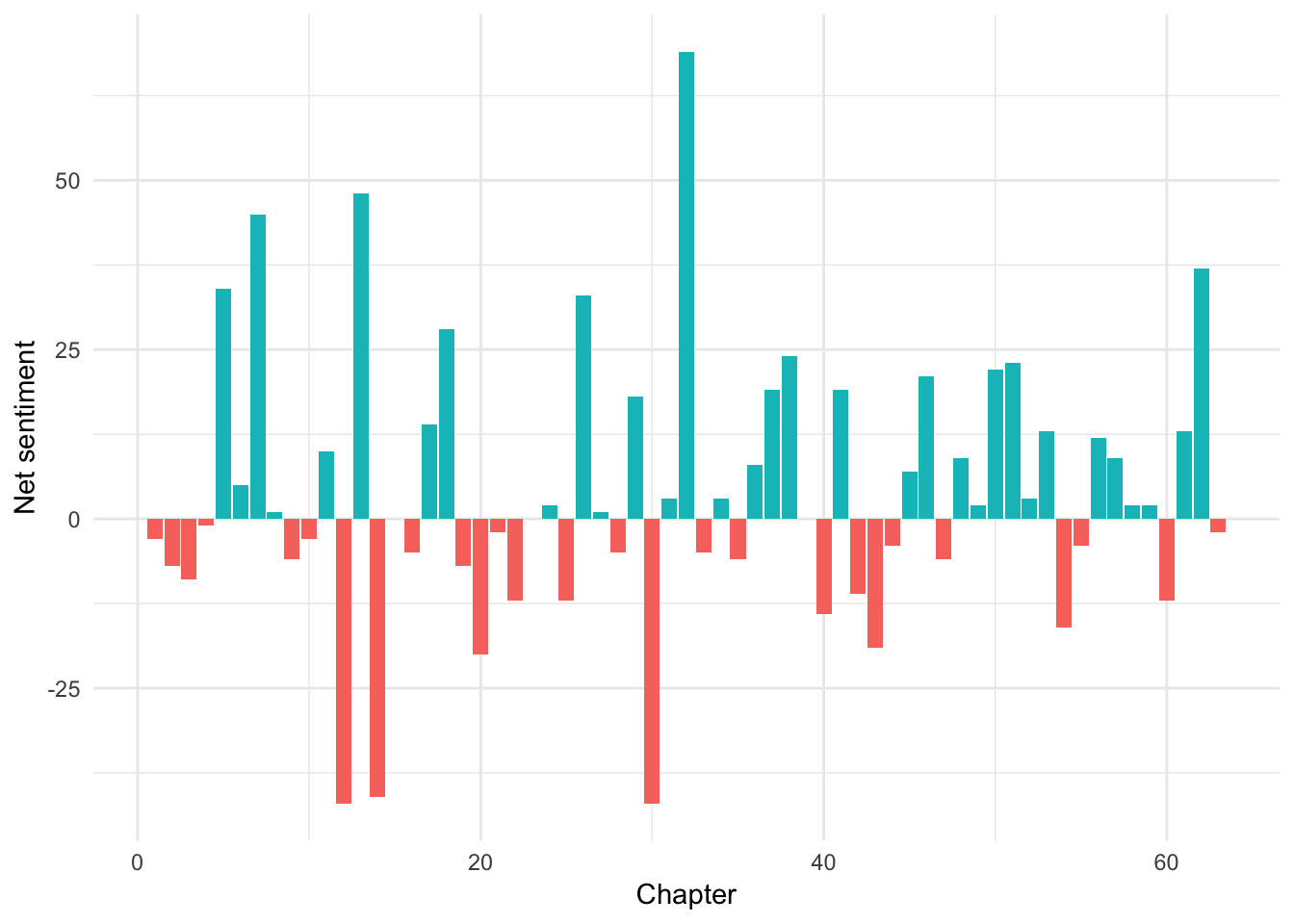

tf-idf

We can determine which words are the most unique for each book/document in our corpus using by calculating the tf-idf (term frequency-inverse document frequency) score for each term. The tf-idf is the product of the term frequency and the inverse document frequency:

\[ \begin{aligned} tf(\text{term}) &= \frac{n_{\text{term}}}{n_{\text{terms in document}}} \\ idf(\text{term}) &= \ln{\left(\frac{n_{\text{documents}}}{n_{\text{documents containing term}}}\right)} \\ tf\text{-}idf(\text{term}) &= tf(\text{term}) \times idf(\text{term}) \end{aligned} \]

Fortunately you don’t need to remember that formula. The bind_tf_idf() function will calculate this for you. Remember, the higher the tf-idf number, the more unique the term is in the document, but these numbers are meaningless and unitless—you can’t convert them to a percentage or anything.

For the sake of space, here are the most unique words in the 4 books of Nephi (I don’t want to try to fit 15 facets on this website)

# Get a list of words in all the books
bom_words <- bom %>% 
  unnest_tokens(word, scripture_text) %>% 
  count(book_title, word, sort = TRUE) %>% 
  ungroup()

# Add the tf-idf for these words
bom_tf_idf <- bom_words %>% 
  bind_tf_idf(word, book_title, n) %>% 
  arrange(desc(tf_idf))

# Get the top 10 uniquest words in just the Nephi books
bom_tf_idf_plot <- bom_tf_idf %>% 
  filter(str_detect(book_title, "Nephi")) %>% 
  group_by(book_title) %>% 
  top_n(10) %>% 
  ungroup() %>% 
  mutate(word = fct_inorder(word))

ggplot(bom_tf_idf_plot, aes(x = fct_rev(word), y = tf_idf, fill = book_title)) +
  geom_col() +
  guides(fill = FALSE) +
  labs(y = "tf-idf", x = NULL) +
  facet_wrap(~ book_title, scales = "free") +
  theme_minimal() +
  coord_flip()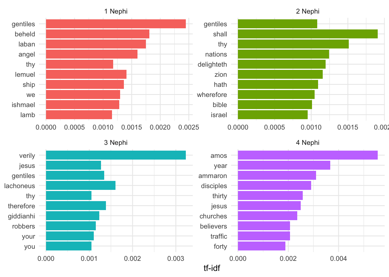

Topic modeling

With topic modeling, we go beyond just counting words and we do some cool unsupervised Bayesian machine learning to find a number of clusters of words that tend to hang together.

dickens_dtm <- dickens %>%
  unnest_tokens(word, text) %>%
  # Get rid of stop words
  anti_join(stop_words) %>%
  count(title, word, sort = TRUE) %>%
  # Convert this to a document-term matrix (a strange data format that LDA nees to work)
  cast_dtm(title, word, n)

# Find 10 topics (or clusters of words)
dickens_lda <- LDA(dickens_dtm, k = 10, control = list(seed = 1234))

# Convert the LDA object into a data frame that we can work with
# The beta column is essentially a measure of word importance within the
# topic---the higher the number, the more important the word is in the topic
dickens_topics <- tidy(dickens_lda, matrix = "beta")

The algorithm finds 10 clusters of words that should be statistically meaningful. In real life, you’d need to determine how these words are related and give them a human-readable name.

# Here are the most important words in each of the 10 clusters
dickens_top_terms <- dickens_topics %>%
  filter(!is.na(term)) %>% 
  group_by(topic) %>%
  top_n(10, beta) %>%
  ungroup() %>%
  arrange(topic, -beta)

# Make a comma separated list of the top 10 terms in each topic
dickens_top_terms %>% 
  group_by(topic) %>% 
  nest(term) %>% 
  mutate(words = data %>% map_chr(~ paste(.$term, collapse = ", "))) %>% 
  select(-data) %>% 
  pander::pandoc.table()

topic	words
1	time, copperfield, home, dear, mind, peggotty, half, mother, aunt, day
2	time, house, head, hand, miss, returned, night, door, pumblechook, day
3	defarge, lorry, miss, time, madame, hand, night, doctor, manette, pross
4	hand, house, dear, hands, night, looked, sir, business, head, returned
5	scrooge, christmas, ghost, spirit, time, cried, bob, scrooge’s, door, hand
6	peggotty, micawber, aunt, miss, time, traddles, agnes, copperfield, dora, mother
7	time, micawber, dear, aunt, traddles, miss, night, steerforth, murdstone, hand
8	lorry, head, sir, father, looked, hand, day, door, tellson’s, red
9	joe, pip, looked, herbert, wemmick, miss, havisham, estella, jaggers, biddy
10	peggotty, returned, miss, aunt, house, micawber, dear, head, agnes, eyes

And here are those 10 topics graphed:

dickens_top_terms %>%
  mutate(term = reorder(term, beta)) %>%
  ggplot(aes(term, beta, fill = factor(topic))) +
  geom_col(show.legend = FALSE) +
  labs(x = NULL, y = "LDA beta (word importance in topic)") +
  theme_minimal() +
  facet_wrap(~ topic, scales = "free") +
  coord_flip()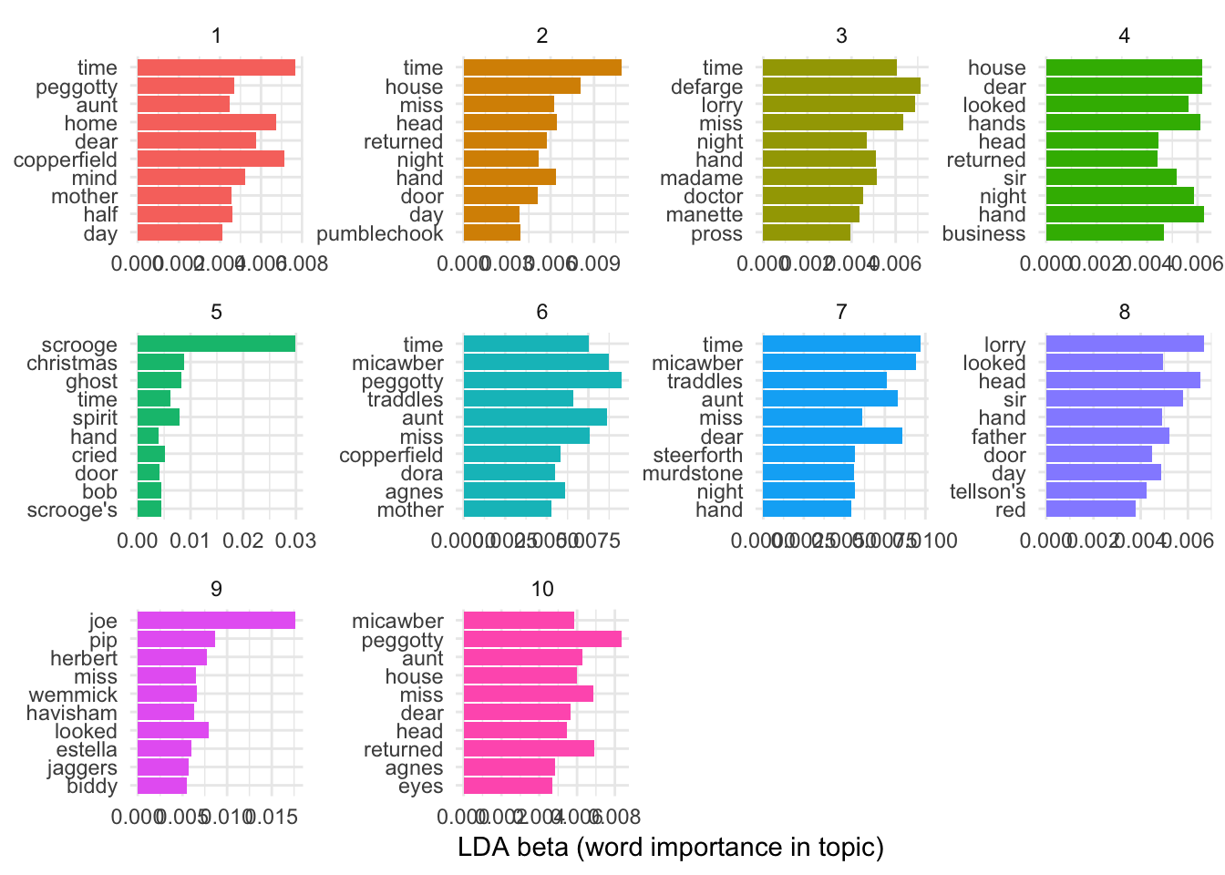

Fingerprinting

Hapax legomena

Finally, we can do some document fingerprinting based on specific text characteristics. First, we’ll look at how often each chapter in the Book of Mormon uses hapax legomena (words that appear only once).

# Count the words in the BoM; make a new variable named hapax that is true if
# the word only appears once
bom_words <- bom %>% 
  unnest_tokens(word, scripture_text) %>% 
  count(word, sort = TRUE) %>% 
  mutate(hapax = n == 1)

# Make a lookup table of BoM chapters. This is helpful because we need to
# combine book names and chapter numbers to get unique hapaxes in each
# book+chapter combination, but then when we plot the results, we still need
# individual non-combined columns for chapter numbers and book names. This makes
# a small data frame of book titles, chapter numbers, and combined book+chapter
bom_lookup <- bom %>% 
  distinct(book_title, chapter_number) %>% 
  mutate(book_chapter = paste0(book_title, " ", chapter_number),
         book_title = as.character(book_title)) %>% 
  mutate(chapter_number = str_remove(book_chapter, book_title),
         chapter_number = as.integer(chapter_number)) %>% 
  mutate(book_title = fct_inorder(book_title))

# Calculate how many hapaxes appear in each chapter of the BoM
bom_hapax <- bom %>% 
  unnest_tokens(word, scripture_text) %>% 
  left_join(bom_words, by = "word") %>% 
  mutate(book_chapter = paste0(book_title, " ", chapter_number)) %>% 
  group_by(book_chapter) %>% 
  summarize(num_words = n(),
            num_hapax = sum(hapax, na.rm = TRUE)) %>% 
  ungroup() %>% 
  mutate(prop_hapax = num_hapax / num_words) %>% 
  left_join(bom_lookup, by = "book_chapter")

As you can see in the plot, the Isaiah chapters in 2 and 3 Nephi use a surprising number of hapaxes, indicating that they probably come from a different author.

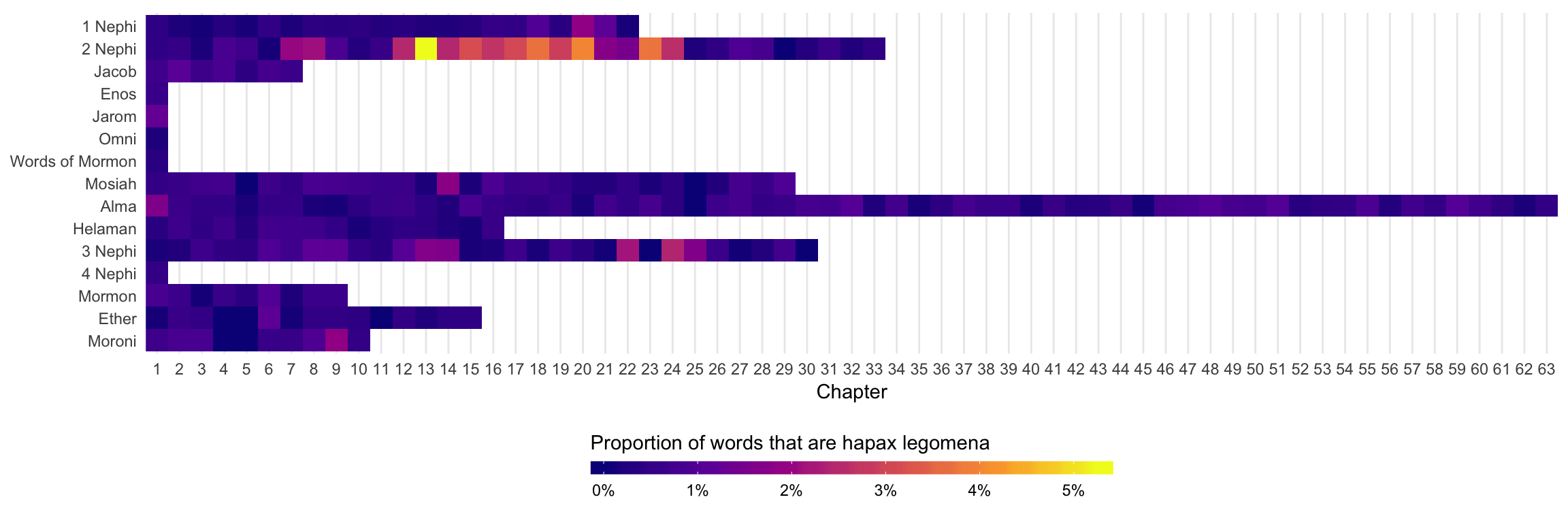
Verse length

We can also make a fingerprint based on verse length. Here we use the Old and New Testaments, just for fun. Job, Psalms, and Proverbs all have really short verses, as do the first few chapters in 1 Chronicles. The verses in Revelation are longer, as are the verses in Hebrew and 2 Peter. The verse length in Luke and Acts appears to be roughly the same.

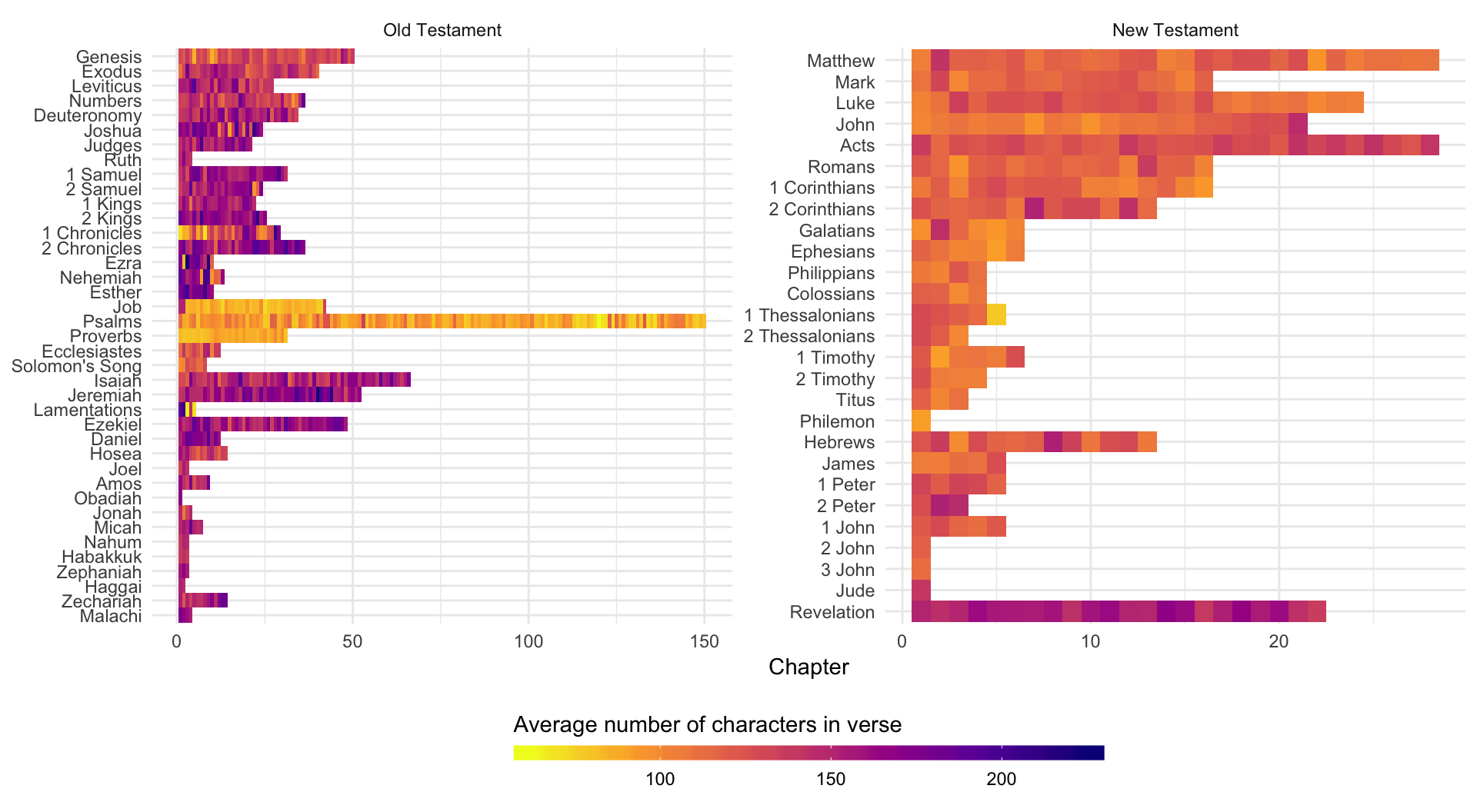
Text features

Finally, we can use the big guns and get all sorts of interesting features for every verse, like the number of punctuation marks, capital letters, periods, etc. using the textfeatures() function:

# For textfeatures() to work, the column with the text in it has to be named text
bom_features <- bom %>% 
  rename(text = scripture_text) %>% 
  # Don't calculate sentiment because it takes a little longer. Also don't
  # calculate word2vec dimensions, since these take longer to do and they're
  # kinda weird and uninterpretable. Also don't normalize the final
  # numbers---keep them as raw numbers
  textfeatures(sentiment = FALSE, word2vec_dims = FALSE, normalize = FALSE) %>% 
  # Add the BoM text back to the data frame, since textfeatures wiped it out
  bind_cols(bom)

# Look at all these columns you can work with now!
glimpse(bom_features)

## Observations: 6,604
## Variables: 31
## $ volume_title     <chr> "Book of Mormon", "Book of Mormon", "Book of ...
## $ n_urls           <int> 0, 0, 0, 0, 0, 0, 0, 0, 0, 0, 0, 0, 0, 0, 0, ...
## $ n_hashtags       <int> 0, 0, 0, 0, 0, 0, 0, 0, 0, 0, 0, 0, 0, 0, 0, ...
## $ n_mentions       <int> 0, 0, 0, 0, 0, 0, 0, 0, 0, 0, 0, 0, 0, 0, 0, ...
## $ n_chars          <int> 304, 104, 97, 251, 114, 178, 134, 213, 114, 9...
## $ n_commas         <int> 7, 2, 0, 6, 5, 1, 1, 4, 1, 1, 2, 1, 7, 7, 4, ...
## $ n_digits         <int> 0, 0, 0, 0, 0, 0, 0, 0, 0, 0, 0, 0, 0, 0, 0, ...
## $ n_exclaims       <int> 0, 0, 0, 0, 0, 0, 0, 0, 0, 0, 0, 0, 1, 2, 0, ...
## $ n_extraspaces    <int> 0, 0, 0, 0, 0, 0, 0, 0, 0, 0, 0, 0, 0, 0, 0, ...
## $ n_lowers         <int> 288, 97, 89, 235, 105, 172, 128, 204, 109, 90...
## $ n_lowersp        <dbl> 0.9475410, 0.9333333, 0.9183673, 0.9365079, 0...
## $ n_periods        <int> 1, 1, 1, 1, 1, 1, 1, 1, 1, 1, 1, 1, 1, 0, 1, ...
## $ n_words          <int> 68, 25, 27, 56, 28, 46, 33, 46, 30, 20, 35, 1...
## $ n_caps           <int> 6, 4, 5, 6, 3, 2, 3, 4, 2, 1, 1, 3, 7, 8, 3, ...
## $ n_nonasciis      <int> 0, 0, 0, 0, 0, 0, 0, 0, 0, 0, 0, 0, 0, 0, 0, ...
## $ n_puncts         <int> 2, 0, 2, 3, 0, 2, 1, 0, 1, 0, 1, 0, 4, 3, 1, ...
## $ n_capsp          <dbl> 0.02295082, 0.04761905, 0.06122449, 0.0277777...
## $ n_charsperword   <dbl> 4.420290, 4.038462, 3.500000, 4.421053, 3.965...
## $ n_polite         <dbl> 0.0000000, 0.0000000, -0.2500000, 0.0000000, ...
## $ n_first_person   <int> 2, 2, 3, 1, 1, 0, 0, 0, 0, 0, 1, 0, 2, 1, 2, ...
## $ n_first_personp  <int> 0, 0, 0, 0, 0, 0, 0, 0, 0, 0, 0, 0, 0, 0, 0, ...
## $ n_second_person  <int> 0, 0, 0, 0, 0, 0, 0, 0, 0, 0, 0, 0, 0, 0, 0, ...
## $ n_second_personp <int> 0, 0, 1, 2, 3, 2, 3, 2, 3, 1, 1, 2, 2, 2, 2, ...
## $ n_third_person   <int> 0, 0, 1, 2, 1, 0, 1, 2, 1, 2, 2, 1, 1, 3, 0, ...
## $ n_tobe           <int> 2, 0, 1, 2, 0, 0, 1, 2, 1, 0, 0, 1, 2, 2, 1, ...
## $ n_prepositions   <int> 2, 2, 2, 5, 4, 4, 4, 4, 5, 2, 4, 3, 4, 4, 4, ...
## $ volume_title1    <chr> "Book of Mormon", "Book of Mormon", "Book of ...
## $ book_title       <fct> 1 Nephi, 1 Nephi, 1 Nephi, 1 Nephi, 1 Nephi, ...
## $ chapter_number   <int> 1, 1, 1, 1, 1, 1, 1, 1, 1, 1, 1, 1, 1, 1, 1, ...
## $ verse_number     <int> 1, 2, 3, 4, 5, 6, 7, 8, 9, 10, 11, 12, 13, 14...
## $ scripture_text   <chr> "I, Nephi, having been born of goodly parents...

Clearest and muddiest things

Go to this form and answer these two questions:

What was the muddiest thing from class today? What are you still wondering about?
What was the clearest thing from class today? What was the most exciting thing you learned?

I’ll compile the questions and send out answers after class.